Semantic Distillation: A Brief Primer

The fact that business teams are drowning in disconnected data is getting to be a bit of a cliche. Adding a semantic layer to an enterprise data platform can bring order to chaos, allowing teams to collaborate effectively and leverage AI to unlock valuable insights. My company, Kobai, has been working to make this technology more accessible, scaleable and easy to adopt. In this article we introduce Semantic Distillation, a new technology designed to rapidly generate and populate semantic models, automating the mapping of source data without losing the ability for teams to embed their own knowledge and point of view into the process. It is the key enabler of Kobai Precursor, currently in private Beta.

Semantic Layers are Great

By putting a familiar face on your data — your own terminology — semantic layers make it discoverable, understandable and reusable. They increase the number of people who can work with it, enabling subject matter experts, not just developers, more efficient access to information when key decisions need to be made.

When those semantic layers are powered by knowledge graphs, they’re even better. The flexibility of a graph better accommodates the complexity of large organizations, allowing the model itself to maximize comprehension by humans without the confusing hacks usually required to shoehorn a company’s collective knowledge into the capabilities of relational databases.

This is all more important, not less, with the advent of chat AI models, and the retrieval techniques they use to incorporate your data into their responses. Trained on massive volumes of human generated text (ie. The Internet), they thrive on context. The data itself is useful, but the database schema or json structure it lives in is a poor substitute for a semantic explanation. This is why data platforms are increasingly emphasizing “description” or “comment” fields when defining schema — no longer as documentation to help the next developer writing SQL code, but as context for the Text2SQL or RAG workflow.

Barriers to Adoption

In our experience with customer engagements, building the initial semantic model is intuitive for subject matter experts, not much more complex than sketching the key components of a given domain on a whiteboard. The hard part is connecting the data, especially as the semantic model evolves and grows, and new data sources are added over time. There are various approaches to this challenge, some better than others, but they all have one thing in common: actually making connections between data entities (tables, columns, documents, fields, etc) and the elements in your semantic model (classes, properties, relationships). Like an old-timey telephone switchboard operator, each piece of source data must have its wire plugged into the correct socket.

Make Sure It’s YOUR Model

We certainly aren’t the first to propose methods of automating the data mapping activity, and with the rise of LLMs they increasingly revolve around “letting AI build the model”. This is medicine that causes more critical symptoms than it cures. When we say we want a Semantic Model, what we implicitly mean is we want a “My Semantics” Model. If the purpose of this model is to make data more understandable to your team, or to help AI interpret questions posed by your team, it should express your data in the terminology that gets thrown around in YOUR team meetings, not somebody else’s.

Who cares what ChatGPT thinks we should call it?!?

Kobai does a lot of work in the aviation industry. If an AI looked at their data and comes up with the perfectly cogent description “sub-assembly”, that really wouldn’t jive with a team using the aviation specific lingo “line replaceable unit”. In this case, not only are we missing out on a much more familiar term of art in aviation, but have also introduced a subtle shift in meaning. Things get even more complicated with hierarchies within the model or relationships between objects. There are usually multiple ways to group or organize a model, but often only one way that matches how a given team actually DOES think about their data.

These methods throw the baby out with the bathwater. In attempting to automate the labour intensive data mapping, they have forfeited the ability for humans to ensure the model matches their view of the world.

Enter Semantic Distillation

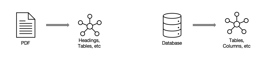
At its core, semantic distillation is a method to integrate models. Any model, really. For our use case, we’ll recognize that data sources contain their own rudimentary models, albeit focused on machine efficiency rather than human consumption. Database tables have an obvious structure, but even Wikipedia pages or PDF documents can be interpreted as models, with structural hints provided by headings, paragraph structure, etc.

To retain the all-important human guidance over the semantic model, we will also feed into the process a partial model defined by our own team. This model can be a partial starting point, focused on the most important concepts for your business. This will guide, but not limit, the distillation process, and the resulting model may contain suggested extensions to the model that the users can choose to incorporate (or not).

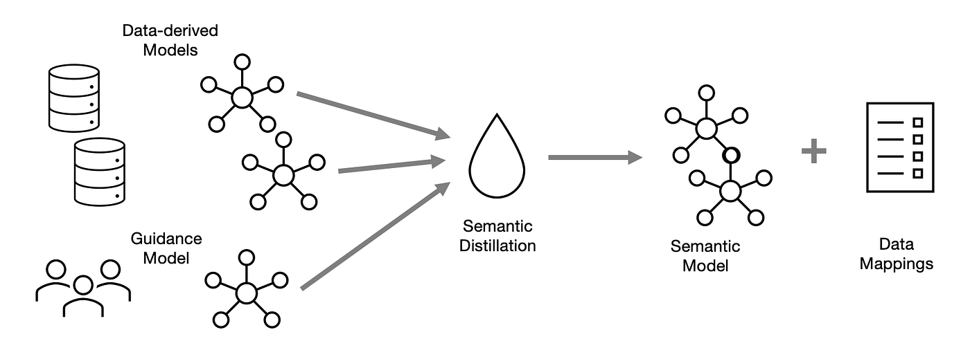
When we take multiple models and put them through this distillation, we should expect that the resulting model has better semantics — that is, a better description and contextualization of its parts — because it has the benefit of multiple expressions of similar concepts from the source models. While the mechanism is different, it is similar in concept to how reading multiple newspapers might give a reader a more complete understanding of the day’s news.

It Takes a (Contextual) Neighbourhood

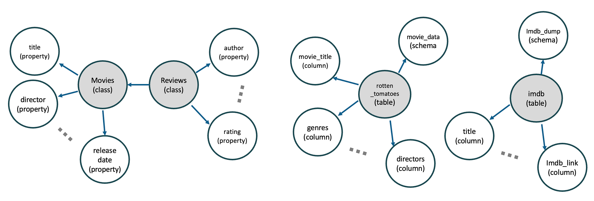
Looking across our guidance model and the models extracted from our data sources, we see different types of entities: Classes and properties in the human-derived models, and things like tables and columns in the data-derived models. On their own, each of these things may only have a simple label telling us not very much at all. If we’re going to really understand these elements, we need to look around a bit.

We call this the contextual neighbourhood, and the ingredients vary by what is available. From a semantic model, we can find properties attached to classes, neighbouring classes, parent classes, etc. From a database, each table can be associated with metadata like column names and schema names, and also profiling information extracted from data samples. A property “temperature” tells me something very different if I know it belongs to a class called “human vital signs” versus one called “conference room”. A column “name” means virtually nothing at all until you find out whether the table name is “movies” or “movie reviewers”.

A Brief Note on Examples: To introduce semantic distillation in as simple a manner as possible, we will keep the examples quite simple. The text above might imply that we’re assuming data source tables are the only option to be compared to classes in the guidance model — this is certainly not the case. Breaking down data sources into objects can benefit, for example, from profiling the data as well, adding not only metadata to the available context, but also breaking down tables into column groupings that may make better matches for other sources or the guidance model itself. While we hope this article serves as a brief primer, future posts will dig into juicier details in this regard.

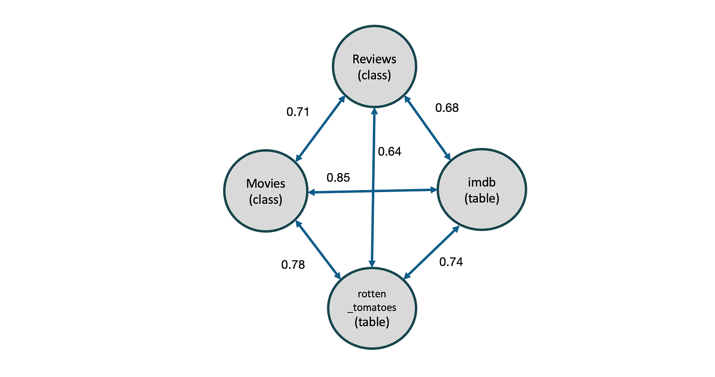
Semantic distillation starts with the question “How similar are these things?”. To answer, we will use the contextual neighbourhoods for each object to compare it to all the other objects. We first summarize each neighbourhood by encoding each element with an LLM, and combining the resulting vectors using a weighted sum.

Now we can put all of those into a graph with weighted edges. To do this, we need to evaluate the distance between every pair of vectors. This is the same math carried out when we ask a vector store for the top-k matches for an embedded query string, except at a much larger scale. The RAG problem essentially scales linearly with the number of vectors in the index. Here, our comparison scales with the number of vectors squared. Luckily, we’re implementing this on a Databricks backend.

For those who have spent any time looking at GraphRAG, there are some parallels here. GraphRAG creates unweighted connections between entities, and then uses a community finding algorithm to divide them into likely communities. In the next step, we will use a method that will divide all the entities into groups/communities based on much more sensitive contextual information, as represented by the vector similarity scores computed above.

Another Brief Aside: Does this really help? In a recent project, we used semantic compression to extract a semantic model from brownfield data belonging to a large process plant. It contained a hierarchical tree of assets that had labels like “NEY 578 A” and “KUT 423 C” (changed to anonymize the data). As it turns out, these are asset tags built using a local convention, with zero information about what kind of equipment they actually represent. The data came from an XML structure, so our context neighbourhood included properties belonging to the equipment, which in turn tied to templates with pretty predictable names: “Temperature”, “Pressure”, “Sump Diameter”, etc. As a guidance model, we were using a standard ISO maintenance model used in the Oil & Gas industry. During the compression process, we achieved a nice match with “Centrifugal Pump” in the guidance model.

Levels of Analysis

Is a similarity score of 0.5 a lot? 0.8? 0.99? How similar is similar? The answer, predictably, is “it depends”. To illustrate, here is a simple example. Let us consider three real world objects:

• a Toyota Corolla
• a Ford F150 pickup truck
• a Sikorsky Sky Crane helicopter.

How similar are these objects? Well, at one level of analysis (perhaps the most obvious level) they are completely different: a passenger car, a work truck, and a heavy-lift flying machine.

However, at another level of analysis, they are exactly the same: they are all vehicles that move from point A to point B.

Which level of analysis is correct? Depends on the user and the use case. If you recall here that our ultimate goal is the creation of a semantic model for a particular team, then it becomes obvious that we need to capture a wide variety of groupings, at all levels. If we add an intermediate case where the two four-wheeled vehicles are more similar to each other than they are to the helicopter, and remember that models can contain parent classes, this gets more interesting.

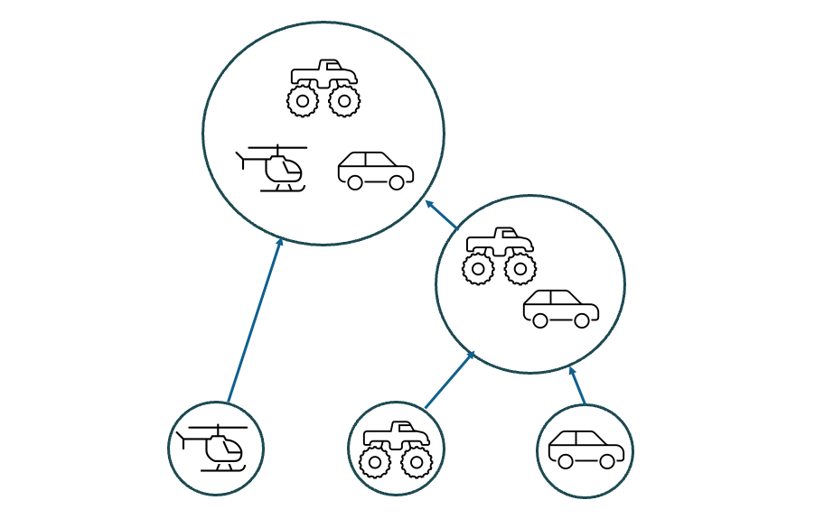
Going back to our movie example from above, we can generate a similar hierarchical grouping of tables by iteratively evaluating our similarity graph against a list of confidence levels. In reality, we apply some frequency analysis to determine the most useful intervals to use, but for the sake of argument, let’s try these values: [0.5, 0.6, 0.7, 0.8, 0.9]

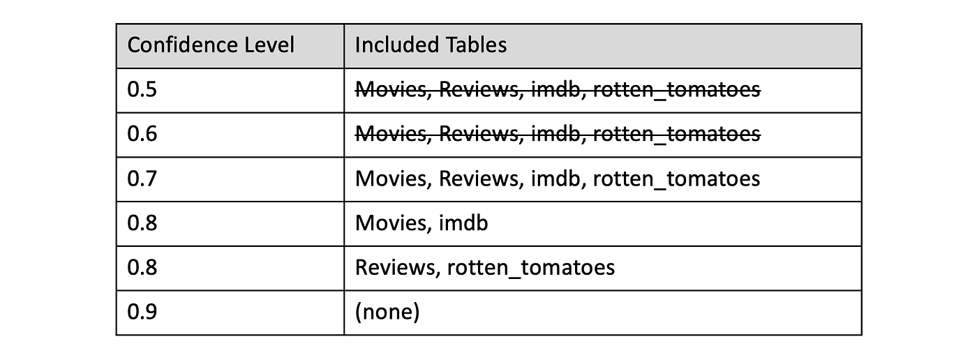
After removing some redundant groups, we have a tree of potential groupings incorporating elements of our guidance model and data source models. For some arbitrary level of confidence, the elements within these groups appear to be the same. This means they’re potential classes for our resulting semantic — potential because we can still apply some additional selection to make sure these align with what our team is looking for.

Class Action

To narrow down the list, we can start by selecting any groups containing exactly one guidance model class, as this was the model we’ve been asked to adhere to. We could also choose to reject any groups containing more than one guidance model class, as these represent more abstraction than the guidance calls for.

When we want to consider classes outside the guidance model (or where no guidance model is provided), we can provide an interface for the user to make case by case selections and/or use metrics to select the “best” classes. Kobai Precursor provides a simple user interface for capturing these preferences.

Finally, Some Names!

We set out here to populate a semantic model with human guidance, so we should use the guidance model where possible. In the case where the semantic class contains exactly one class from the guidance model, we can name the new class by simply taking the name of the guidance model class verbatim.

For all other cases, we build a context neighbourhood graph at the highest level, and give that to an LLM prompt. This generates an appropriate name from the accumulated context in the prospective semantic model, including the names of properties, adjacent classes, parents, etc.

Let’s See It In Action

What shall we do with our newly refined semantic model and associated data mapping rules? Whatever we want, really. One example provided out of the box by Kobai Precursor is deploying the model to Kobai Studio, with pre-populated mapping rules.

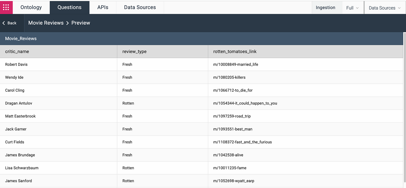
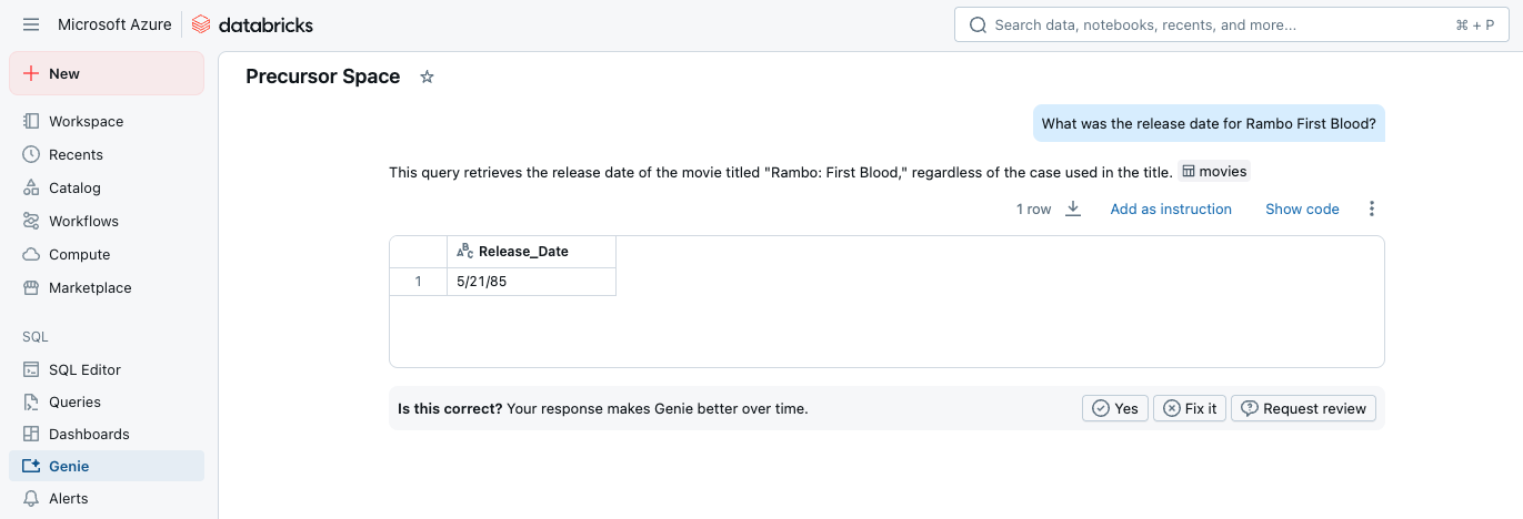
Another good place to start would be publishing to Databricks’ Unity Catalog. After that one-click operation in Precursor, we can write a quick query to see what our favourite reviewer has to say.

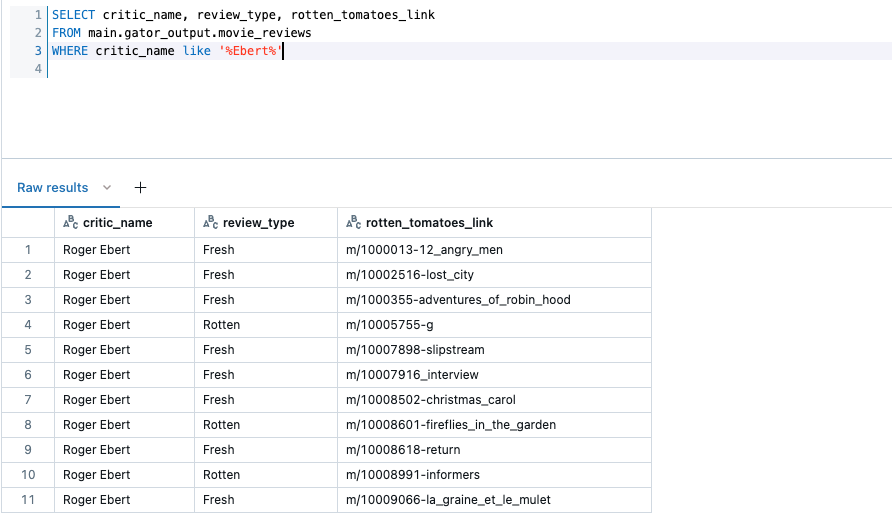
Taking it one step further, we could use Kobai’s integration with Databricks Genie to make it even easier.

Powerful Use Cases

Imagine a manufacturing company with multiple data sources — ERP systems, quality control data from sensors, and production data. Semantic Distillation can seamlessly integrate these data sources, even when they use different terminology for the same concept, like ‘raw materials’ and ‘input components.’ The technology automatically groups similar terms together, creating a unified semantic model that makes data accessible and actionable for everyone in the organization — without the need for extensive technical expertise.

While this core “data mapping” use case uses data sources and a guidance model as inputs, that is far from the only application for semantic distillation. Other use cases include:

• Rapid deployment of analytics to industrial fleet data, where the off-the-shelf analytic has an implied model for inputs that may not match the user’s structures.
• Configuration of data for consumption by AI/LLM query capabilities, allowing GraphRAG approaches with the same velocity as basic unstructured RAG.
• On-boarding of brownfield fleet data into a standard interface. For example, industrial sites configured independently are difficult to compare analytically, and labour intensive to map into a standardized ontology.

Going Deeper

In future articles, we will delve into semantic distillation in much more detail, and pickup some threads we left dangling here.

• How we use the same distillation process to generate properties for our new classes.
• How we manage identifiers when mapping different data sources representing the same real-world objects.

Thanks for reading! To learn more about Semantic Distillation and Kobai Precursor, reach out to us at https://www.kobai.io